Kaggle: Digit Recognition

So this blog post is actually going to be a little different because this has nothing to do with GSOC(Google Summer of Code) but well it could because some of the projects have to deal with NLP(Natural Language Processing) but for now we will be dealing with a competition relating to digit recognition. So essentially we want to teach the computer to be able to read handwritten digits. The images generated are a 28 * 28 image that is in greyscale. Now working on the project was myself Keanu Nichols and Akil Hosang we used a Neural Network approach and we tried to model it after the Coursera Machine Learning (ML) course by Andrew Ng. We did a very simple implementation by the way, it was for us to simply work on a problem since we were working on the ML course and wanted to get some actual experience working on a project so we looked to Kaggle and one of the beginner projects was this. Overtime I hope we can improve the score of this approach which I believe is possible. So let’s dive into it.

First we go about importing our different modules as seen below, pandas is used for dataframes to store the pixels of the images and do a number of different operations. Matplotlib is used to actually see the image using the dataframes storing the pixels. Numpy is used to manipulate array to do things like transposing a matrix or multiplying two matrices. Random is used to give random numbers as will be seen in the function “randInit”. And finally minimize which is an equivalent to fmincg in matlab which is used to train the actual Neural Network.

# Plot ad hoc mnist instances
import pandas as pd
import matplotlib.pyplot as plt
%matplotlib inline
import numpy as np
import pandas as pd
import random
import math
from scipy.optimize import minimize

Then we go onto loading our data into a training set

# load (downloaded if needed) the Kaggle dataset
train = pd.read_csv('./datasets/train.csv')
train.head()

	label	pixel0	pixel1	pixel2	pixel3	pixel4	pixel5	pixel6	pixel7	pixel8	...	pixel774	pixel775	pixel776	pixel777	pixel778	pixel779	pixel780	pixel781	pixel782	pixel783
0	1	0	0	0	0	0	0	0	0	0	...	0	0	0	0	0	0	0	0	0	0
1	0	0	0	0	0	0	0	0	0	0	...	0	0	0	0	0	0	0	0	0	0
2	1	0	0	0	0	0	0	0	0	0	...	0	0	0	0	0	0	0	0	0	0
3	4	0	0	0	0	0	0	0	0	0	...	0	0	0	0	0	0	0	0	0	0
4	0	0	0	0	0	0	0	0	0	0	...	0	0	0	0	0	0	0	0	0	0

5 rows × 785 columns

and test set.

test = pd.read_csv('./datasets/test.csv')
test.head()

	pixel0	pixel1	pixel2	pixel3	pixel4	pixel5	pixel6	pixel7	pixel8	pixel9	...	pixel774	pixel775	pixel776	pixel777	pixel778	pixel779	pixel780	pixel781	pixel782	pixel783
0	0	0	0	0	0	0	0	0	0	0	...	0	0	0	0	0	0	0	0	0	0
1	0	0	0	0	0	0	0	0	0	0	...	0	0	0	0	0	0	0	0	0	0
2	0	0	0	0	0	0	0	0	0	0	...	0	0	0	0	0	0	0	0	0	0
3	0	0	0	0	0	0	0	0	0	0	...	0	0	0	0	0	0	0	0	0	0
4	0	0	0	0	0	0	0	0	0	0	...	0	0	0	0	0	0	0	0	0	0

5 rows × 784 columns

Since we would want to just have the pixels we take the first column and onwards to get all the pixel data and store it in X_train. We then store the labels of the numbers for e.g. if the number is 2 or 3 and we store that in y_train. After we train our test date into X_test, we will actually feed this to the Neural Network and get our outputs and submit to Kaggle.

X_train = (train.iloc[:,1:].values.astype('float32'))
y_train = (train.iloc[:,0].values.astype('int32'))
X_test = test.values.astype('float32')

Now the order in which I do this will not be the exact format of the jupyter notebook but this is for us to better understand the order in which it is executed. So the first part is to store our data into the Neural Network class.

nn = Neural_Network(X_train,np.transpose(y_train))

The Neural_Network class looks like this and we see that it’s initialized with m the number of inputs which in our case will be 784 (28 * 28) our input layer is set to 784, hidden layer is 25 (was used in the exercise for the ML course) and our output layer size is 10 (because we have 10 digits 0-9). Epsilon is what we’re going to calculate soon enough. J is our cost function and grad is our gradient. Num_labels I think is self explanatory the number of labels and lambda1 is lambda which will be used in both forward and back propagation, iter is used when we are going through using minimize for us to see our iteration number of training the Neural Network.

class Neural_Network:
   #The Neural_Network class we use to store all the values that
   #will be used to teach our model to start recognizing handwritten
   #digits
   def __init__(self,X,y):
       self.m = X_train.shape[0]
       self.input_layer_size = X_train.shape[1]
       self.hidden_layer_size = 25
       self.output_layer_size = 10
       self.epsilon = []
       self.J = 0
       self.grad = 0
       self.num_labels = 10
       self.lambda1 = 0
       self.iter = 0

So we go forward actually getting theta1 (for our pixels) and theta2 (for our number labels). We will call the function “randInit()” to actually populate it with values.

theta1 = theta2 = []
theta1,theta2 = nn.randInit()

We first go out getting our values for epsilon, which was given by the ML course (under Random Initialization), we split it for theta1 and theta2 that’s why epsilon is a list of two values. We also add our bias unit. We then store our values for theta1 and theta2 by random initialization. It is more or less using what’s in the course.

   def randInit(self):
       theta1 = []
       theta2 = []
       for x in range(2):
           if(x == 0):
               L_in = self.input_layer_size
               L_out = self.hidden_layer_size
           if(x == 1):
               L_in = self.hidden_layer_size
               L_out = self.output_layer_size
           self.epsilon.append(math.sqrt(6) / math.sqrt(L_in + L_out))
          
       X_bias = self.input_layer_size + 1
      
       theta1 = (np.random.rand(self.hidden_layer_size,
                self.input_layer_size + 1) * (2 * self.epsilon[0])
                - self.epsilon[0])
       theta2 = (np.random.rand(self.output_layer_size,
                 self.hidden_layer_size + 1) * (2 * self.epsilon[1])
                 - self.epsilon[1])
       return theta1,theta2

The next part is the go ahead and actually train the Neural Network. As seen below we first format the values of theta1 and theta2 and store it so we can use it in different parts of the program, I also used it because the function we will be using called minimize which actually trains the Neural Network want theta1 and theta2 to be store in this format so we store it in nn_params (line 1). The next step is to actually go ahead and train the network (line 2).

nn_params = np.concatenate((theta1.reshape(theta1.size, order='F'), theta2.reshape(theta2.size, order='F')))
theta1,theta2 = nn.train(theta1,theta2,nn_params,X_train,np.transpose(y_train),0.08)

So as we see here train is used to better adjust the values of theta1 and theta2. So we will be using the function minimize which will be using the function nnCostFunction and that will return the cost and gradient each time. Minimize actually is able to detect if the cost function is decreasing and if it isn’t it will adjust accordingly.

def train(self,theta1,theta2,nn_params, X, y, lambda_reg):
       print(self.J)
       print('Training Neural Network...')
       maxiter = 20
       #maxiter = 30
       #maxiter = 60
       #maxiter = 5
       #lambda_reg = 0
       nn_params = np.concatenate((theta1.reshape(theta1.size, order='F'), theta2.reshape(theta2.size, order='F')))
       myargs = (self.input_layer_size, self.hidden_layer_size, self.num_labels, X, y, lambda_reg)
       results = minimize(self.nnCostFunction, x0=nn_params, args=myargs, options={'disp': True, 'maxiter':maxiter}, method="L-BFGS-B", jac=True)

       nn_params = results["x"]

       # Obtain Theta1 and Theta2 back from nn_params
       Theta1 = np.reshape(nn_params[:self.hidden_layer_size * (self.input_layer_size + 1)], \
                        (self.hidden_layer_size, self.input_layer_size + 1), order='F')

       Theta2 = np.reshape(nn_params[self.hidden_layer_size * (self.input_layer_size + 1):], \
                        (self.num_labels, self.hidden_layer_size + 1), order='F')

       print('Program paused. Press enter to continue.\n')
       return Theta1,Theta2

So we will look at the nnCostFunction the first part is to computer forward propagation. We first unpack nn_params and then add a bias unit to both theta1 and theta2. We then go about calculating the activation function from the input layer to the hidden layer and then we do it for the hidden layer to the output layer. We then create a create a matrix that will have 10 labels and will have 0’s in all positions except one which will have 1 which represents what digit the pixels form. We then can calculate the cost function we also use regularization to stop overfitting.

def nnCostFunction(self,nn_params, input_layer_size, hidden_layer_size, \
                      num_labels, X, y, lambda_reg):
      
       self.J = 0;
       self.iter+=1;
       self.lambda1 = lambda_reg

      
       theta1 = np.reshape(nn_params[:hidden_layer_size * (input_layer_size + 1)], \
                    (hidden_layer_size, input_layer_size + 1), order='F')

       theta2 = np.reshape(nn_params[hidden_layer_size * (input_layer_size + 1):], \
                    (num_labels, hidden_layer_size + 1), order='F')
      
       Theta1_grad = np.zeros( theta1.shape )
       Theta2_grad = np.zeros( theta2.shape )
      
       a1 = np.column_stack((np.ones((self.m,1)), X))
      
       z2 = np.dot(a1, theta1.T)
      
       a2 = self.sigmoid(z2)
      
       a2 = np.column_stack((np.ones((a2.shape[0],1)), a2))
      
       z3 = np.dot(a2, theta2.T)
      
       a3 = self.sigmoid(z3)

       numLabels_temp = y
  
       yMatrix = y
       yMatrix = np.zeros((self.m,self.num_labels))
      
       for i in range(self.m):
           yMatrix[i, numLabels_temp[i]-1] = 1
           
       cost = 0
      
       for i in range(self.m):
           cost +=  np.sum( yMatrix[i] * np.log(a3[i]) + (1 - yMatrix[i]) * np.log(1 - a3[i]) )
          
       sqTheta1 = np.sum(np.sum(theta1[:,1:]**2))
       sqTheta2 = np.sum(np.sum(theta2[:,1:]**2))
      
       self.J = -(1.0/self.m) * cost
      
       self.J = self.J + ( (lambda_reg/(2.0*self.m)) *(sqTheta1 + sqTheta2) )
          
       print( str(self.iter) + ") ",self.J," cost")

The next step is to do back propagation, so we go ahead and use values we had gotten from the feedforward calculations and use that to better adjust our theta values and we then store that in ‘self.grad’. We do this for 20 iterations, however this can be increased. There starts to become a point where it does not matter how many iterations you do since the values don’t change by much, which happened with our model. This may have been due to overfitting or underfitting, this is a simple model but later we hope to improve on it and do some analysis on what is happening by using for example cross validation.

#Back Prop
       delta1 = 0;
       delta2 = 0;
       for t in range(0,self.m):
           #print(a1.shape)
           a1_t = a1[t,]
          
           a2_t = a2[t,].T
          
           a3_t = a3[t,].T
          
           y_output_t = yMatrix[t,].T
          
           delta3_t = (a3_t - y_output_t);
          
           z2_t = np.dot(a1_t, theta1.T);
           z2_t= np.insert(z2_t,0 ,1, axis=0)
          
           delta2_t = np.dot(theta2.T, delta3_t) * self.sigmoidGradient(z2_t)
          
           delta2_t = delta2_t[1:]
          
           delta2 = delta2 + np.outer(delta3_t, a2_t)
           delta1 = delta1 + np.outer(delta2_t, a1_t.T)
      
       Theta1_grad = delta1 / self.m
       Theta2_grad = delta2 / self.m
      
       Theta1_grad_unregularized = np.copy(Theta1_grad)
       Theta2_grad_unregularized = np.copy(Theta2_grad)
       Theta1_grad += (float(self.lambda1)/self.m)*theta1
       Theta2_grad += (float(self.lambda1)/self.m)*theta2
       Theta1_grad[:,0] = Theta1_grad_unregularized[:,0]
       Theta2_grad[:,0] = Theta2_grad_unregularized[:,0]
       self.grad = np.concatenate((Theta1_grad.reshape(Theta1_grad.size, order='F'), Theta2_grad.reshape(Theta2_grad.size, order='F')))
       #print(Theta2_grad)
       return self.J,self.grad

Our next step is the begin to predict what numbers are represented in our training set.

pred = nn.predict(theta1, theta2, X_train)

We then compare that to the labels in our training set, as discussed before this may cause a problem with overfitting. We have a accuracy of 76% which to be honest by today’s standards doesn’t seem too great but one step at a time!

k = 0
print(pred[k])
for i in pred:
   if(i == 10):
       pred[k] = 0
   k+=1
print('Training Set Accuracy: {:f}'.format( ( np.mean(pred == y_train)*100 ) ) )

We then use our model to go ahead and predict for the test set and then we just upload that to the Kaggle website. You will see in the file that we had to do some adjusting since for example the model would predict 10 but this is actually 0.

ans = nn.predict(theta1,theta2, X_test)

k = 0
print(ans[1])
for i in ans:
   if(i == 10):
       ans[k] = 0
   k+=1
print(ans[1])

df = pd.DataFrame(data=ans,columns=["Label"])
file = "submission0.csv"
df.reset_index(level=0, inplace=True)
#df['ImageId'] = df.index
df.columns = ['ImageId', 'Label']
for i in df['ImageId']:
   df['ImageId'][i]+=1
#for
print(df[:5])
df.to_csv(file, index=False)

digit = X_test.reshape(X_test.shape[0],28,28)
print(ans[0])
plt.subplot(221)
plt.imshow(digit[i], cmap=plt.get_cmap('gray'))

2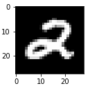

Our best score on Kaggle is 0.87914 but this can definitely be increased through different models.

Resources: Coursera to python

Andrew Ng Machine Learning

Files Used:
Jupyter Notebook - digit_recognizer_blog_code